Join-count analysis is a type of point pattern analysis in which the points are divided into two or more categorical (nominal) classes. It can be thought of as a type of covariance or correlogram analysis of point patterns. A “join” is literally a connection (or edge) between two points. Two points can be joined via a connections matrix or by being a certain distance apart.
The principle of join-counts is fairly simple. Assume that the points fall into just two classes, A and B. Join-count analysis works by looking at all pairs of points that are joined, counting the number of BB pairs (for example) and testing whether the count of BB pairs is more or less than would be expected by chance given the total number of A’s and B’s, and the number of pairs of points within the class. A similar approach may be used to look at AA pairs and AB pairs. This is easily extended to cases in which the points fall into more than two classes.
The joins are defined by an n x n weight matrix, W, where n is the number of points. W is a form of a connections matrix, in which each entry within the matrix, wij, describes whether points i and j are joined or not. Normally, wij = 1 if two points are joined and 0 if they are not, although other weighting schemes can be used (such as weights equal to the inverse of the distance among the points), particularly when an investigator has an a priori hypothesis about distributions they wish to test (Jumars et al. 1977). Rather than computing the join-count statistics for a single weight matrix, one often uses a series of matrices defining different spatial relationships among the points (e.g., distance classes consisting of points separated by successively longer distances) and calculates the statistic for each matrix. See correlogram analysis for more on this.
The expected values and variances of these statistics can be calculated under two sampling assumptions (Cliff and Ord 1973, 1981; Sokal and Oden 1978a): with and without replacement. In the first, one assumes that sampling occurs from a large population and that the probability that a point will be of type r is pr. For the second assumption (sampling without replacement), one assumes that the proportion of localities of type r is pr, but that the number of localities is fixed so that the probability of a location being of type r is conditional on the number of localities of type r that have previously been sampled. Generally, the latter assumption (sampling without replacement) is considered more biologically realistic because most biological populations are finite in size and spatially structured.
The number of joins of the same type (r) can be calculated as
![]()
where ![]() indicates the double
sum over all i and all j, i
≠ j, and f(ri,rj)
equals 1 if points i and j are both of type r
and zero otherwise. Assuming sampling with replacement, the expected number
of joins is
indicates the double
sum over all i and all j, i
≠ j, and f(ri,rj)
equals 1 if points i and j are both of type r
and zero otherwise. Assuming sampling with replacement, the expected number
of joins is
![]()
with variance
 ,
,
where nr
is the number of points of type r,
![]() (the sum of the values in the weight
matrix),
(the sum of the values in the weight
matrix),
![]() ,
,
![]() ,
,
and ![]() and
and ![]() are the sums of the ith
row and ith
column of the weight matrix, respectively.
are the sums of the ith
row and ith
column of the weight matrix, respectively.
The above equations are for joins of the same type; the number of joins of two different types (r and s) is
![]()
where ![]() equals 1 if point
i is of type r
and point j is of type s (or vice versa) and zero otherwise.
The expected number of joins between types r
and s is
equals 1 if point
i is of type r
and point j is of type s (or vice versa) and zero otherwise.
The expected number of joins between types r
and s is
![]() ,
,
with variance
 .
.
Finally, if there are more than two types, the number of total joins between all possible different types is
![]() ,
,
where k is the number of types. The expected number of joins
![]() ,
,
with variance
 .
.
All of the above assumes sampling with replacement. If instead, one assumes sampling without replacement, the expected number of joins of the same type is
![]() ,
,
with variance
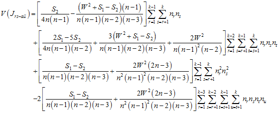
 ;
;
the expected number of joins between types r and s is
![]() ,
,
with variance
 ;
;
and the expected number of joins between all different types is
![]() ,
,
with variance
 .
.
See Cliff and Ord (1973, 1981), Sokal and Oden (1978a), and Dale (1999) for more information on join-count analyses.
| Menu: | Analysis→Point Data→Join-Counts |
| Button: | |
| Batch: | JoinCounts |

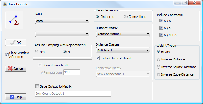
Join-Count analysis window
To perform a join-count analysis in PASSaGE you specify the data matrix and column containing the types. You then choose whether to base the Join-Count classes on distances and distance classes or on a connections matrix. In the former case, you specify the distance matrix and distance classes, and PASSaGE will produce a join-count analysis for every class (there is an option for excluding the largest class). If you choose a connections matrix, PASSaGE will produce a join-count analysis for the single class defined by the connection scheme.
You must also specify the type of contrasts you wish to perform. There are three options: A/A, A/B, and A/Not A. As described above, the first estimates join-counts for all pairs of the same type. The second estimates join-counts for all pairs of different specific types. The third estimates join-counts for all pairs between one type and all other types. This is best illustrated with an example. Assume we have three types: X, Y, and Z. Each option will perform the following contrasts:
| A/A: | X vs. X |
| Y vs. Y | |
| Z vs. Z | |
| A/B: | X vs. Y |
| X vs. Z | |
| Y vs. Z | |
| (X vs. Y) & (X vs. Z) & (Y vs. Z) (all possible non-matching pairs) | |
| A/Not A: | X vs. Y or Z |
| Y vs. X or Z | |
| Z vs. X or Y |
Other options include specifying whether you wish to assume sampling
with or without replacement and the type of weight system you wish to
use. Most join-count analyses are performed using binary weights (1 =
in class, 0 = not in class), but distance-based weighting is also an option.
In distance based-weighting, data points which are closer together have
higher weights than those farther apart, even within the class. If the
distance between points i and
j is dij then the weight
is either ![]() ,
, ![]() ,
or
,
or ![]() depending on whether inverse, inverse
square-, or inverse cube-distance weighting is chosen.
depending on whether inverse, inverse
square-, or inverse cube-distance weighting is chosen.
Significance of join-count statistics can be obtained directly through the expected values and variances, but one can alternatively choose to perform a permutation test. In this test, the distances (locations) among all of the points are maintained, but the types are randomly shuffled across each the locations. This allows one to test whether a specific type of association is significant, conditional on the locations of individuals being fixed.