 ,
,A second metric (a squared-difference coefficient) from Geary (1954) is:
 ,
,
where yi
is the value of the variable at the ith location, n
is the number of points, wij is a weight
indicating something about the spatial relationship of points i
and j, ![]() indicates
the double sum over all i and
all j where i
≠ j, and
indicates
the double sum over all i and
all j where i
≠ j, and ![]() ,
the sum of the values in the weight matrix.
,
the sum of the values in the weight matrix.
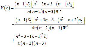
Geary’s c ranges from zero to infinity, with an expected value of 1 under no autocorrelation. Values from zero to one indicate positive spatial autocorrelation, values above 1 negative spatial autocorrelation. As with Moran’s I, we can estimate the variance of Geary’s c under two sampling assumptions. Assuming that the observed data could be randomly permuted across all of the observed locations, the variance of c can be estimated as
 ,
,
with S1, S2, and b2 defined as for Moran’s I. Assuming an infinite, normally distributed variable, the variance can be estimated as
![]() .
.
Geary’s c is closely related to semivariogram analysis; a Geary's c correlogram is essentially a standardized semivariogram. Moran’s I and Geary’s c usually yield similar interpretations; differences between them are described in Sokal (1979).