Contiguous three-dimensional data matrices are difficult to display in two dimensions since the interior data is masked by the exterior surfaces. PASSaGE includes two methods for plotting data of this type: Surface and Post.
| Menu: | Draw→Plot→3D/Cube |
| Button: | |
| Batch: | <none> |
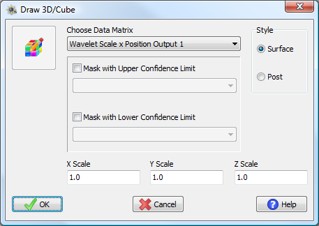
Draw 3D/Cube window.
A 3D surface plot draws two-dimensional slices of the data as if it were a surface plot. The user has direct control of whether the slice is being cut through the x-, y-, or z-axis, and can specify the position along the axis to make the slice. The plot is “live” such that the position is controlled dynamically while graphed and does not need to be specified in advance, allowing the user to move back and forth along a given axis. A description of these options can be found under Special Options for 3D Surface Plots.
(A)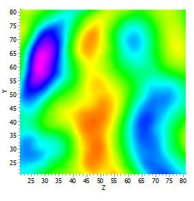 (B)
(B)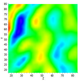
(C)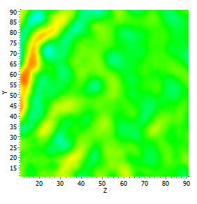 (D)
(D)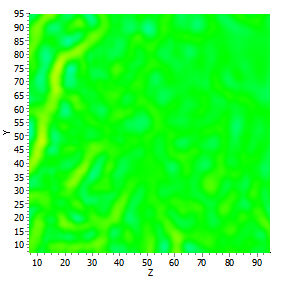
Examples of graphed 3D data matrix, drawn as a surface plot. Each plot represents a different surface layer sliced from the 3D data. All of these represent the Y/Z plane, taken from different values of X. (A) X = 10; (B) X = 8; (C) X = 5; (D) X = 3. The data comes from a two-dimensional wavelet analysis of the elevation surface; the Y/Z plane represents the positions of the surface; the different X slices represent different scales, while color indicates the magnitude of the variance for that scale × position combination.
A 3D post plot is a three-dimensional representation of the volume, which can be rotated to any viewing angle in real time. Every cell within the volume is represented by a small colored sphere. This is an anti-space filling representation: the spheres are purposefully spread out to allow one to view through the volume (if it were space-filling one would only see the outside surfaces). These plots are graphically interesting, but can be computationally consuming if the 3D volume to be plotted is large.

Examples of graphed 3D data matrix, drawn as a post plot. The same wavelet data as in the previous figure. The X-axis (across the page, left to right) represents the scale, while each plane represents positions on the original surface.
The colors of both of these plots are controlled through standard gradation controls. Scale and masking options are available for 3D plots and work identicaly to those for drawing surfaces.